NZ Electricity Generation
covid 19 lockdown v1.0
Ben Anderson, Carsten Dortans and Marilette Lotte
Last run at: 2020-07-10 16:35:27
1 About
1.1 Citation
1.2 Report circulation
- Public – this report is intended for publication
1.3 Code
All code used to create this report is available from:
1.4 License
This work is made available under the Creative Commons Attribution-ShareAlike 4.0 International (CC BY-SA 4.0) License.
This means you are free to:
- Share — copy and redistribute the material in any medium or format
- Adapt — remix, transform, and build upon the material for any purpose, even commercially.
Under the following terms:
- Attribution — You must give appropriate credit, provide a link to the license, and indicate if changes were made. You may do so in any reasonable manner, but not in any way that suggests the licensor endorses you or your use.
- ShareAlike — If you remix, transform, or build upon the material, you must distribute your contributions under the same license as the original.
- No additional restrictions — You may not apply legal terms or technological measures that legally restrict others from doing anything the license permits.
Notices:
- You do not have to comply with the license for elements of the material in the public domain or where your use is permitted by an applicable exception or limitation.
- No warranties are given. The license may not give you all of the permissions necessary for your intended use. For example, other rights such as publicity, privacy, or moral rights may limit how you use the material.
For the avoidance of doubt and explanation of terms please refer to the full license notice and legal code.
1.5 History
1.6 Support
This work was supported by:
- The University of Otago;
- SPATIALEC - a Marie Skłodowska-Curie Global Fellowship based at the University of Otago’s Centre for Sustainability (2017-2019) & the University of Southampton’s Sustainable Energy Research Group (2019-2020).
- The European Union via SPATIALEC, a Marie Skłodowska-Curie Global Fellowship based at the University of Otago’s Centre for Sustainability (2017-2019) & the University of Southampton’s Sustainable Energy Research Group (2019-2020) (Anderson);
- The Uniersity of Otago via a Centre for Sustainability Summer Scholarship (Lotte) and PhD Studentship (Dortans)
2 Introduction
Building on (???), we are interested in GHG emissions from the NZ electricity generation over time. We are especially interested in how this might change during the NZ covid-19 lockdown period (2020-03-24 to 2020-07-10).
We use two different GHG emissions indicators:
- % of total generation in a halfhour which was ‘low emissions’ where this is defined as wind + solar + hydro
- Calculated CO2e emissions per half hour (not yet implemented)
3 Data
3.1 Wholesale generation data
Essentially ‘grid’ generation from major power stations of various kinds. Data downloaded from https://www.emi.ea.govt.nz/Wholesale/Datasets/Generation/Generation_MD/ and pre-processed.
| Site_Code | POC_Code | Nwk_Code | Gen_Code | Fuel_Code | Tech_Code | Trading_date | Time_Period | kWh | strTime | rTime | rDate | rDateTime | month | year | rDateTimeOrig | rDateTimeNZT | rMonth |
|---|---|---|---|---|---|---|---|---|---|---|---|---|---|---|---|---|---|
| ARA | ARA2201 | MRPL | aratiatia | Hydro | Hydro | 2017-01-01 | TP1 | 11510 | 0:15:00 | 00:15:00 | 2017-01-01 | 2017-01-01 00:15:00 | 1 | 2017 | 2017-01-01T00:15:00Z | 2017-01-01 00:15:00 | Jan |
| ARA | ARA2201 | MRPL | aratiatia | Hydro | Hydro | 2017-01-02 | TP1 | 11570 | 0:15:00 | 00:15:00 | 2017-01-02 | 2017-01-02 00:15:00 | 1 | 2017 | 2017-01-02T00:15:00Z | 2017-01-02 00:15:00 | Jan |
| ARA | ARA2201 | MRPL | aratiatia | Hydro | Hydro | 2017-01-03 | TP1 | 11090 | 0:15:00 | 00:15:00 | 2017-01-03 | 2017-01-03 00:15:00 | 1 | 2017 | 2017-01-03T00:15:00Z | 2017-01-03 00:15:00 | Jan |
| ARA | ARA2201 | MRPL | aratiatia | Hydro | Hydro | 2017-01-04 | TP1 | 13970 | 0:15:00 | 00:15:00 | 2017-01-04 | 2017-01-04 00:15:00 | 1 | 2017 | 2017-01-04T00:15:00Z | 2017-01-04 00:15:00 | Jan |
| ARA | ARA2201 | MRPL | aratiatia | Hydro | Hydro | 2017-01-05 | TP1 | 19680 | 0:15:00 | 00:15:00 | 2017-01-05 | 2017-01-05 00:15:00 | 1 | 2017 | 2017-01-05T00:15:00Z | 2017-01-05 00:15:00 | Jan |
| ARA | ARA2201 | MRPL | aratiatia | Hydro | Hydro | 2017-01-06 | TP1 | 27190 | 0:15:00 | 00:15:00 | 2017-01-06 | 2017-01-06 00:15:00 | 1 | 2017 | 2017-01-06T00:15:00Z | 2017-01-06 00:15:00 | Jan |
##    Fuel_Code          sd
## 1:      Coal  229.305827
## 2:    Diesel    2.377192
## 3:       Gas  396.418119
## 4:       Geo  610.506277
## 5:     Hydro 1888.429777
## 6:      Wind  156.224244
## 7:      Wood   22.686248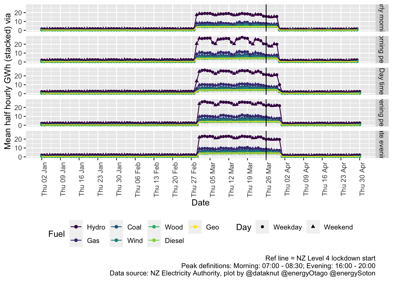
3.2 Embedded generation data
Essentially ‘non-grid’ generation from solar photovoltaic and small scale wind which is ‘embedded’ - i.e. non-grid connected as it is connected ‘downstream’ of the grid exit points (GXP). Data downloaded from https://www.emi.ea.govt.nz/Wholesale/Datasets/Metered_data/Embedded_generation and pre-processed.
| POC | NWK_Code | Participant_Code | Loss_Code | Flow_Direction | Trading_date | Time_Period | kWh | strTime | rTime | rDate | rDateTime | month | year | rDateTimeOrig | rDateTimeNZT | rMonth |
|---|---|---|---|---|---|---|---|---|---|---|---|---|---|---|---|---|
| ASB0661 | EASH | TRUS | H01 | I | 01/01/2017 | TP1 | 0 | 0:15:00 | 00:15:00 | 2017-01-01 | 2017-01-01 00:15:00 | 1 | 2017 | 2017-01-01T00:15:00Z | 2017-01-01 00:15:00 | Jan |
| ASB0661 | EASH | TRUS | H01 | I | 02/01/2017 | TP1 | 0 | 0:15:00 | 00:15:00 | 2017-01-02 | 2017-01-02 00:15:00 | 1 | 2017 | 2017-01-02T00:15:00Z | 2017-01-02 00:15:00 | Jan |
| ASB0661 | EASH | TRUS | H01 | I | 03/01/2017 | TP1 | 0 | 0:15:00 | 00:15:00 | 2017-01-03 | 2017-01-03 00:15:00 | 1 | 2017 | 2017-01-03T00:15:00Z | 2017-01-03 00:15:00 | Jan |
| ASB0661 | EASH | TRUS | H01 | I | 04/01/2017 | TP1 | 0 | 0:15:00 | 00:15:00 | 2017-01-04 | 2017-01-04 00:15:00 | 1 | 2017 | 2017-01-04T00:15:00Z | 2017-01-04 00:15:00 | Jan |
| ASB0661 | EASH | TRUS | H01 | I | 05/01/2017 | TP1 | 0 | 0:15:00 | 00:15:00 | 2017-01-05 | 2017-01-05 00:15:00 | 1 | 2017 | 2017-01-05T00:15:00Z | 2017-01-05 00:15:00 | Jan |
| ASB0661 | EASH | TRUS | H01 | I | 06/01/2017 | TP1 | 0 | 0:15:00 | 00:15:00 | 2017-01-06 | 2017-01-06 00:15:00 | 1 | 2017 | 2017-01-06T00:15:00Z | 2017-01-06 00:15:00 | Jan |
| year | sumkWh_I | sumkWh_X | nObs_I | nObs_X |
|---|---|---|---|---|
| 2017 | 5058591128 | 96830431 | 406372 | 1225680 |
| 2018 | 5069984029 | 121534268 | 527004 | 1577056 |
| 2019 | 5208373429 | 105300995 | 437276 | 1394172 |
| 2020 | 1522565086 | 35504132 | 144624 | 492048 |
Not entirely sure what these codes mean yet. Limited guidance available? TBC
For now embedded generation data is not included in the following analysis.
4 Background trends and patterns
Demand profiles by season
## Saving 7 x 5 in image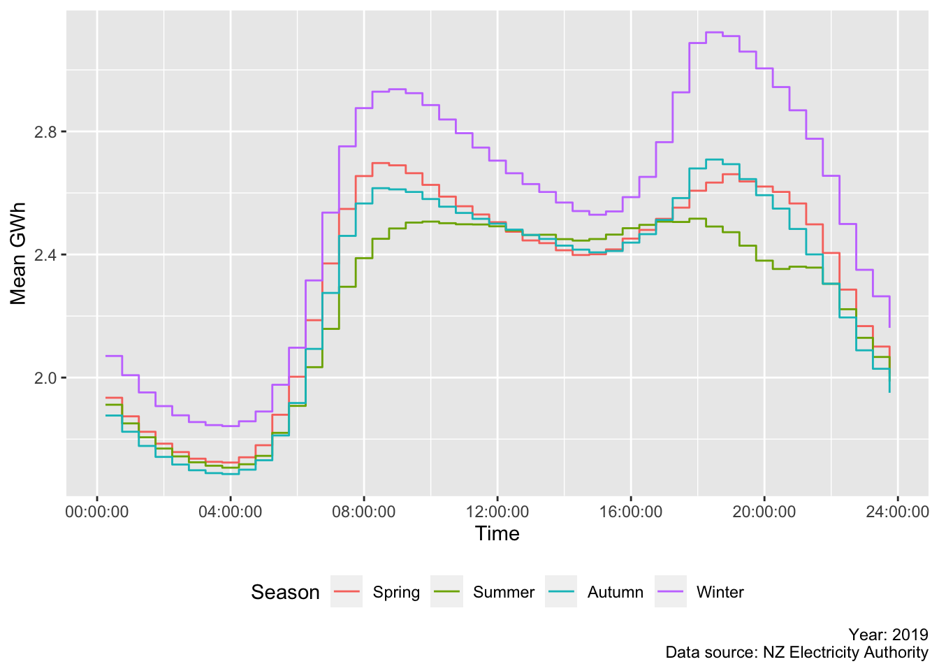
## Warning in checkPrep(mydata, vars, type, remove.calm = FALSE): Detected data with Daylight Saving Time, converting
## to UTC/GMT
## [1] "Taking bootstrap samples. Please wait."
## [1] "Taking bootstrap samples. Please wait."
## [1] "Taking bootstrap samples. Please wait."
## [1] "Taking bootstrap samples. Please wait."
## [1] "Taking bootstrap samples. Please wait."
## quartz_off_screen
## 2| year | Early morning | Morning peak | Day time | Evening peak | Late evening |
|---|---|---|---|---|---|
| 2017 | 1.87 | 2.60 | 2.53 | 2.64 | 2.32 |
| 2018 | 1.86 | 2.61 | 2.53 | 2.65 | 2.32 |
| 2019 | 1.88 | 2.62 | 2.54 | 2.66 | 2.34 |
| 2020 | 5.84 | 7.76 | 7.90 | 8.07 | 7.18 |
5 Analysis (think this section needs some structure/sub-headings!)
In this section we analyse the current developments in electricity generation during the Covid-19 level four alert. The level four alert came into effect on March 25 2020 at 11.59pm as part of the fight agianst the novel Covid-19 virus. The minimum lockdown period is four weeks, ending on April 28 This period has wide-spread implications across New Zealand’s economy and electriicty consumption, amongst other effects such as everyday life in general.
All non-essential busineeses are closed and staff is asked to work from home. This analysis aims to provide insights on developments in electriicty generation. Essential research questions company this research:
To what extent has electricity generation shown deviation of ‘normal’ generation patterns during the level four alert?
Has the composition of fuel sources supplying electriicty demand in New Zealand changed during the level four alert?
Has the level four alert impacted greenhouse-gas emissions associated with electriicty generation?
| nObs | |
|---|---|
| Coal | 19200 |
| Diesel | 19200 |
| Gas | 172800 |
| Geo | 211200 |
| Hydro | 726432 |
| Wind | 172800 |
We extracted electricity generation data from /INSERT DATES/. Table 5.1 shows the number of observations for each fuel type for the aforementioned dates. It becomes clear that Hydro was the most used fuel type, followed by Geothermal, Wind, Gas, Coal, and Diesel.
| Fuel_Code | rDateTimeNZT | Time_Period | rMonth | year | meankWh | sumkWh | nObs | meanMW | sumMW |
|---|---|---|---|---|---|---|---|---|---|
| Coal | 2018-01-01 00:15:00 | TP1 | Jan | 2018 | 102674 | 102674 | 1 | 205.348 | 205.348 |
| Coal | 2018-01-01 00:45:00 | TP2 | Jan | 2018 | 90091 | 90091 | 1 | 180.182 | 180.182 |
| Coal | 2018-01-01 01:15:00 | TP3 | Jan | 2018 | 85373 | 85373 | 1 | 170.746 | 170.746 |
| Coal | 2018-01-01 01:45:00 | TP4 | Jan | 2018 | 84806 | 84806 | 1 | 169.612 | 169.612 |
| Coal | 2018-01-01 02:15:00 | TP5 | Jan | 2018 | 63093 | 63093 | 1 | 126.186 | 126.186 |
| Coal | 2018-01-01 02:45:00 | TP6 | Jan | 2018 | 54723 | 54723 | 1 | 109.446 | 109.446 |
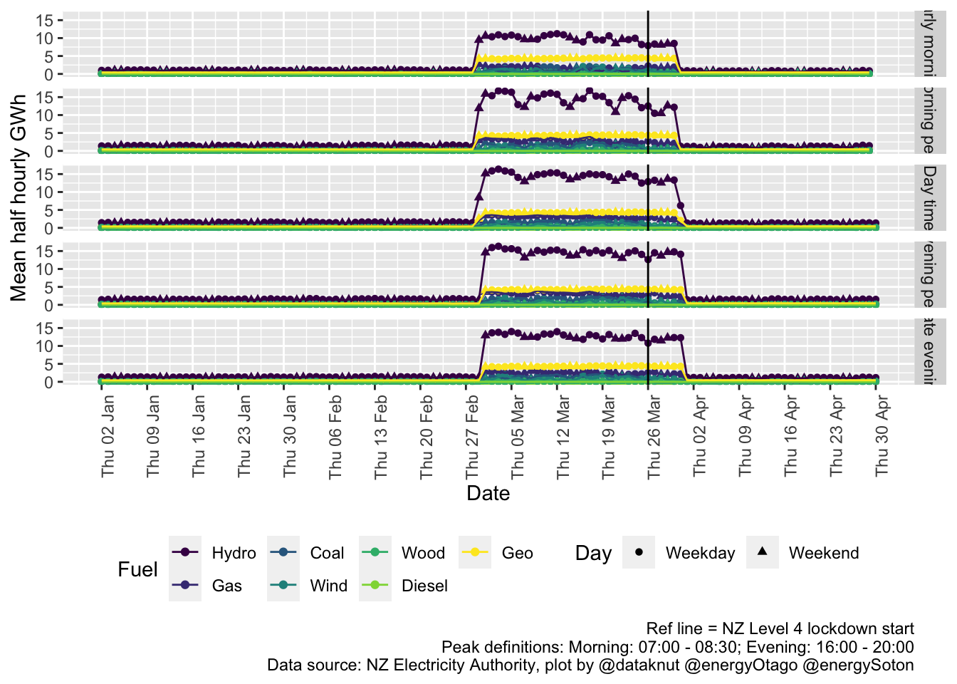
Table 5.2 shows exemplary data of our data extraction. In addition, Figure 5.1 pictures total generation (this is the sum for each fuel type for all generatinfg plants and all trading periods). Hydro had the highest power output in January and February. Geothermnal was used for base load and an increase in Gas output is viible for the second half of February. Wind intermittently generated while Coal was occasionally integrated. Wood and Diesel did not contribute much in January and February.
## `geom_smooth()` using method = 'gam' and formula 'y ~ s(x, bs = "cs")'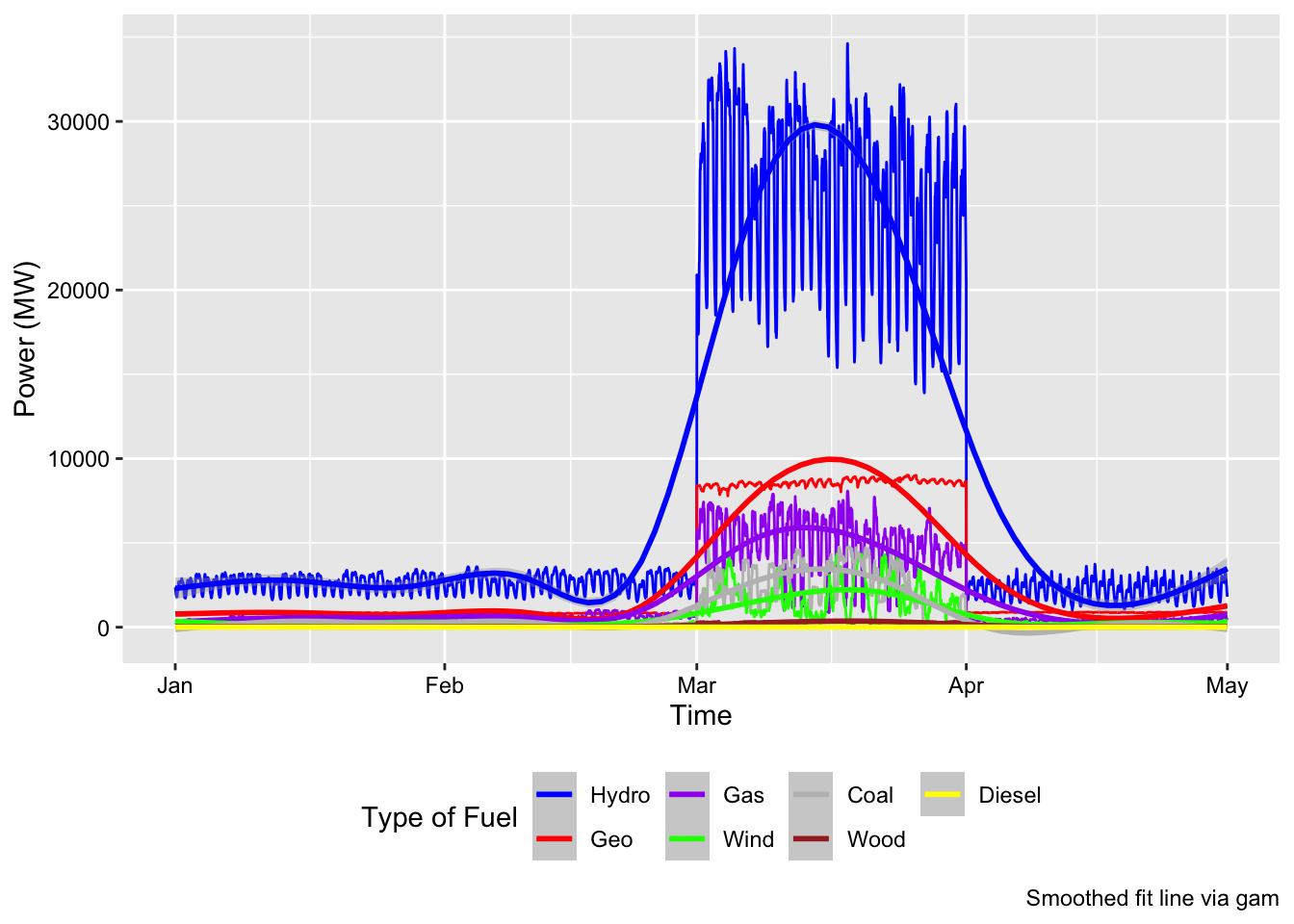
Figure 5.1: Total generation by fuel
Figure 5.2 shows total generation for the first four months of 2020. A red box indicates the alert level four period.
## `geom_smooth()` using method = 'gam' and formula 'y ~ s(x, bs = "cs")'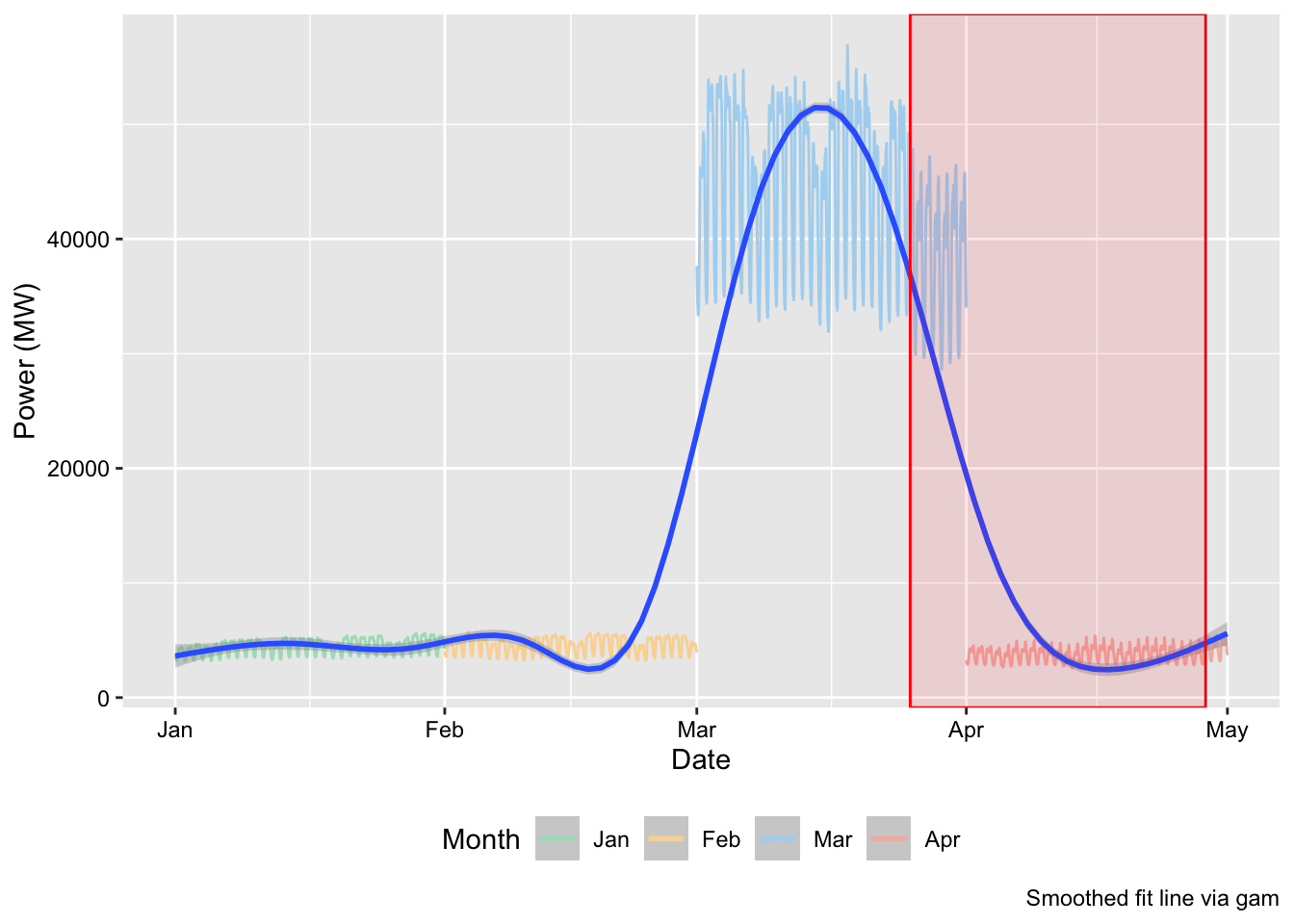
Figure 5.2: Four months of total generation for 2020
## `geom_smooth()` using method = 'gam' and formula 'y ~ s(x, bs = "cs")'In order to provide information on how generation changed over time it is helpful to compare it with previous years. Twenty matching weekdays were extracted for January to March for 2020, 2019, and 2018. We would like to make sure that the weekdays really ‘match up’. Figure 5.3 shows twenty days of extracted data for the three years for March We see that the weekdays match up.
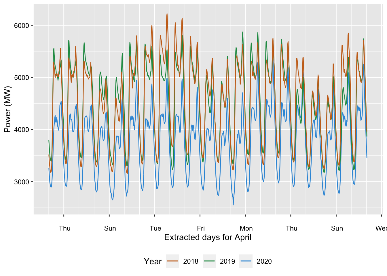
Figure 5.3: Twenty days of total generation for March by year
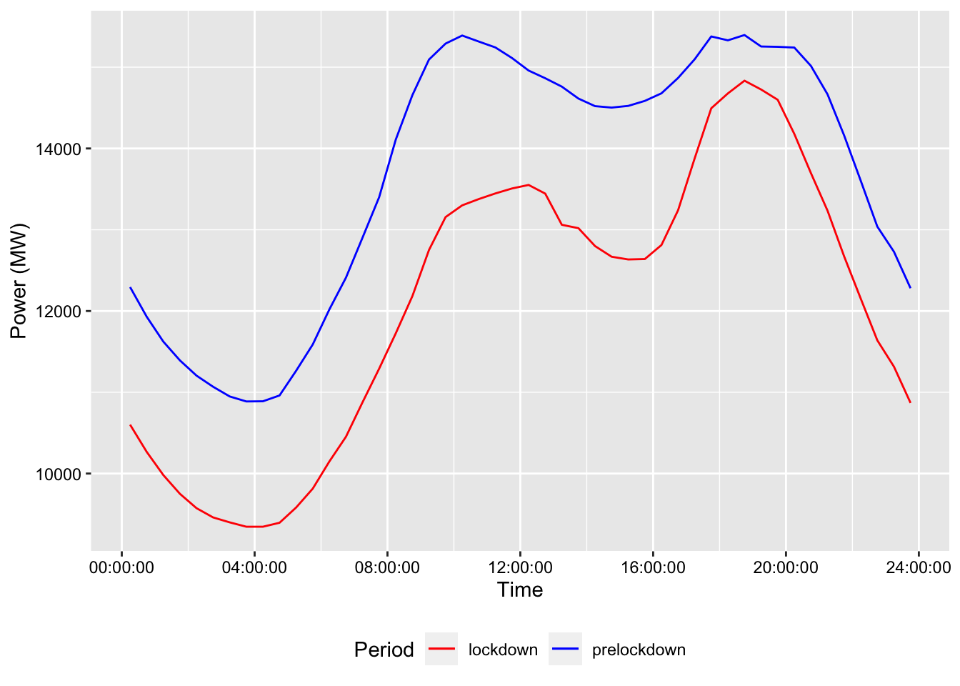
Figure 5.4 shows a close-up for one day in March for the three years. We see that on this particular Saturdays during the lockdown period the morning peak was shifted towards mid-day. Total generation at morning peak dropped by 11% compared to previous years. Interestingly, the evening peak reached almost the same total generation despite the lockdown but was shifted by one hour.
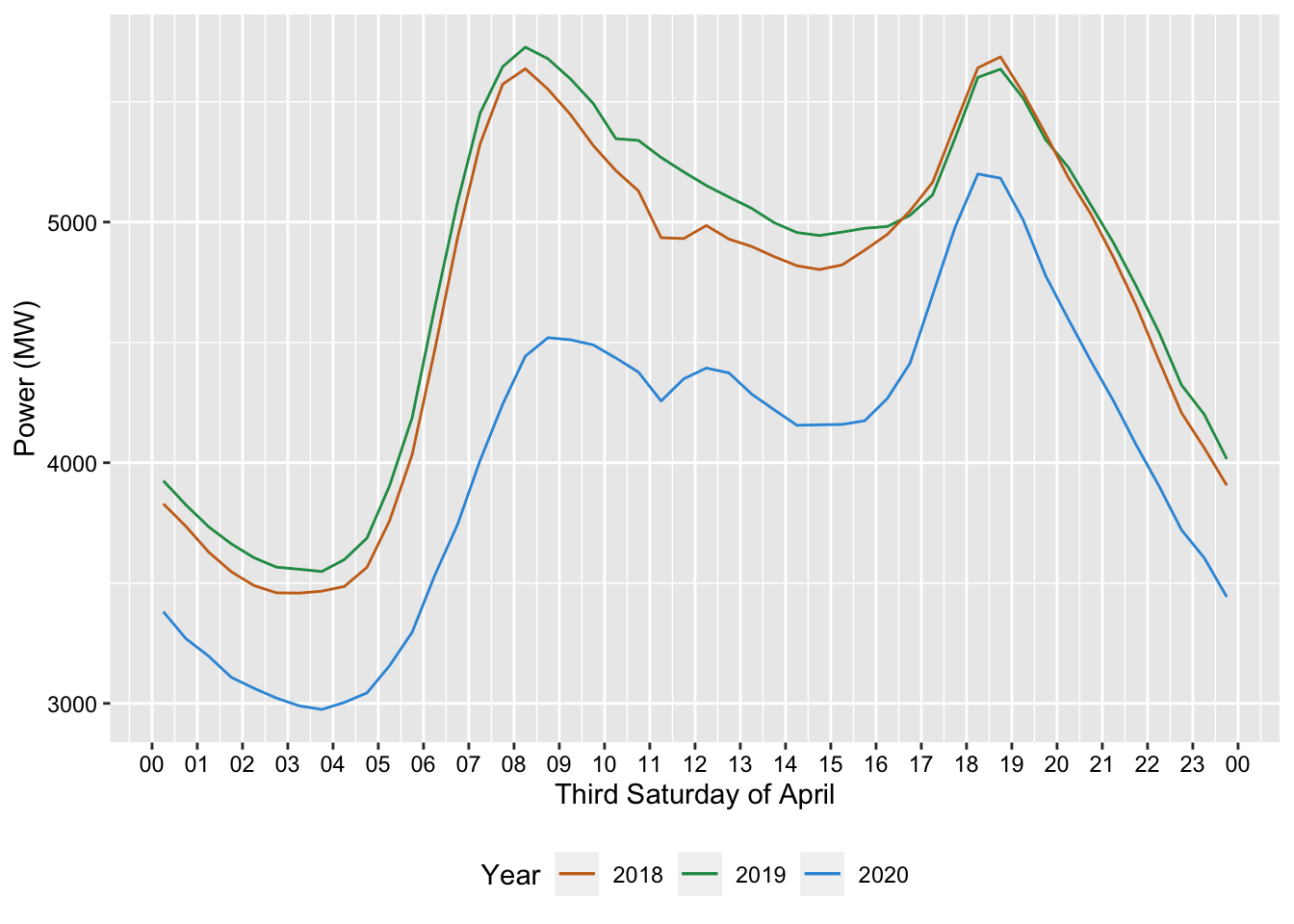
Figure 5.4: Total generation over time for the third Saturday in April by year
A less distorted view on total generation data is provided in Figure 5.5. Instead of 15-minute granularity data daily means represent ttoal generation. We can see how close the analysed years were togetehr before the lockdowm and as the lockdown starts a large rop in generation occurs.
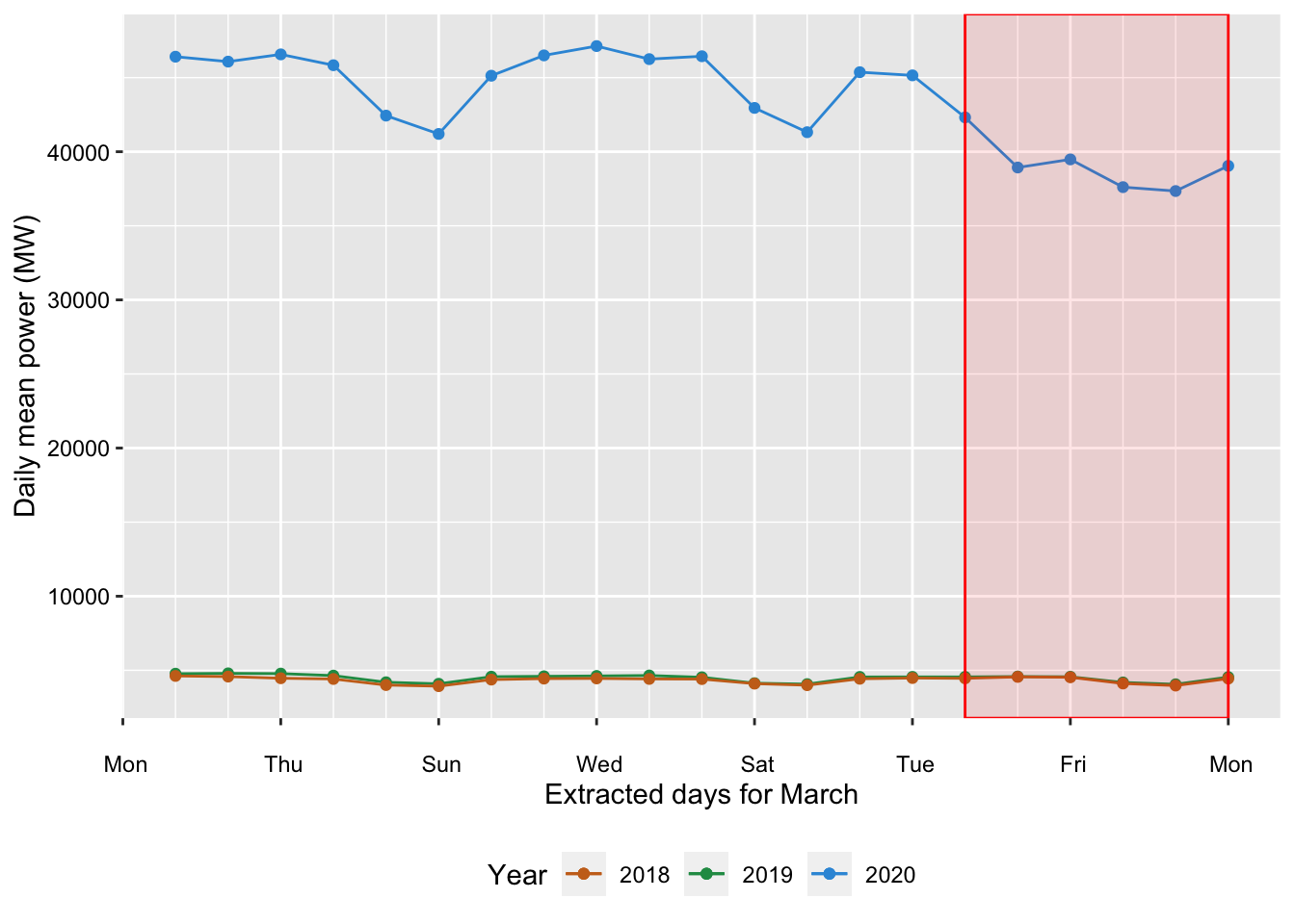
Figure 5.5: Daily mean generation by year for March
A mean over 2018 and 2019 data was compared with 2020 in Figure 5.6. In addition, previous months were considered in this plot as well and show that the variation apparent during the lockdown period is significant between the two reference periods.
Figure 5.7 highlights the percentage difference between 2020 and the reference period of 2018-2019. On a daily mean granularity, generation dropped by over 15% during the lockdown period.
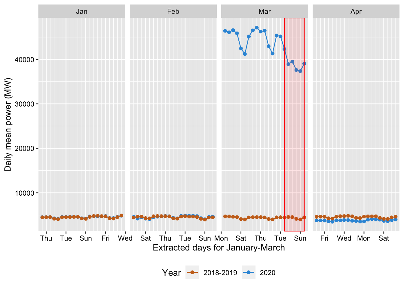
Figure 5.6: Daily mean total generation for 2020 and reference period by month
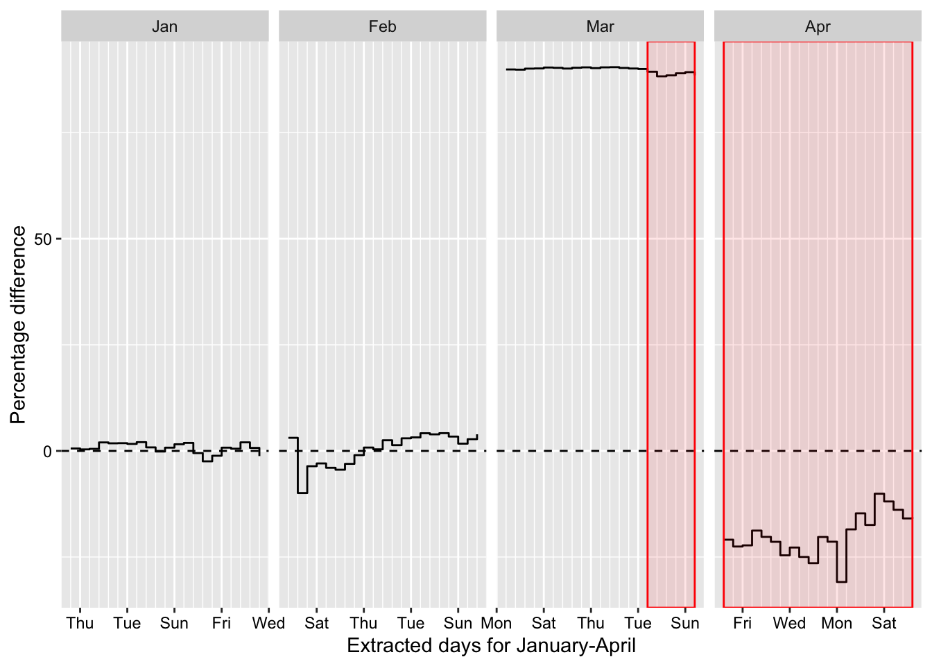
Figure 5.7: Percentage difference in daily mean between 2018-2019 and 2020
Seems to break
This also breaks?
6 Experiments with openair
openair is an R package designed for air quality analysis but it has some useful plots that we can make use of.
For example, Figure ?? uses the openair TheilSen() function (Carslaw and Ropkins 2012) to create a de-seasoned trend plot for mean monthly half-hourly (i.e. the mean of all half-hourly GW values for each month) generation in GW split by weekdays and weekend days. These plots show that there has been a steady decline in generation (and thus demand) over the period.
currently fails as openair needs latticeExtra which needs R (≥ 3.6.0)
7 Annexes
7.1 Wholesale generation data (‘grid’)
| Name | allGridDT |
| Number of rows | 5048944 |
| Number of columns | 19 |
| _______________________ | |
| Column type frequency: | |
| character | 11 |
| difftime | 1 |
| factor | 2 |
| numeric | 3 |
| POSIXct | 2 |
| ________________________ | |
| Group variables | None |
Variable type: character
| skim_variable | n_missing | complete_rate | min | max | empty | n_unique | whitespace |
|---|---|---|---|---|---|---|---|
| Site_Code | 0 | 1 | 3 | 3 | 0 | 61 | 0 |
| POC_Code | 0 | 1 | 7 | 7 | 0 | 61 | 0 |
| Nwk_Code | 0 | 1 | 4 | 4 | 0 | 25 | 0 |
| Gen_Code | 0 | 1 | 3 | 15 | 0 | 63 | 0 |
| Fuel_Code | 0 | 1 | 3 | 6 | 0 | 7 | 0 |
| Tech_Code | 0 | 1 | 3 | 5 | 0 | 5 | 0 |
| Trading_date | 0 | 1 | 10 | 10 | 0 | 1216 | 0 |
| Time_Period | 0 | 1 | 3 | 4 | 0 | 48 | 0 |
| strTime | 0 | 1 | 7 | 8 | 0 | 48 | 0 |
| rDate | 0 | 1 | 10 | 10 | 0 | 1216 | 0 |
| rDateTimeOrig | 0 | 1 | 20 | 20 | 0 | 58356 | 0 |
Variable type: difftime
| skim_variable | n_missing | complete_rate | min | max | median | n_unique |
|---|---|---|---|---|---|---|
| rTime | 0 | 1 | 900 secs | 85500 secs | 43200 secs | 48 |
Variable type: factor
| skim_variable | n_missing | complete_rate | ordered | n_unique | top_counts |
|---|---|---|---|---|---|
| rMonth | 0 | 1 | TRUE | 12 | Mar: 1354176, Jan: 418128, Apr: 405216, Feb: 380832 |
| season | 0 | 1 | FALSE | 4 | Aut: 2074848, Sum: 1112736, Win: 936192, Spr: 925168 |
Variable type: numeric
| skim_variable | n_missing | complete_rate | mean | sd | p0 | p25 | p50 | p75 | p100 | hist |
|---|---|---|---|---|---|---|---|---|---|---|
| kWh | 0 | 1 | 32527.65 | 48455.12 | 0 | 3943.64 | 16470 | 41741 | 402430 | ▇▁▁▁▁ |
| month | 0 | 1 | 5.55 | 3.39 | 1 | 3.00 | 4 | 8 | 12 | ▇▃▂▂▃ |
| year | 0 | 1 | 2018.53 | 1.12 | 2017 | 2018.00 | 2019 | 2020 | 2020 | ▇▇▁▇▇ |
Variable type: POSIXct
| skim_variable | n_missing | complete_rate | min | max | median | n_unique |
|---|---|---|---|---|---|---|
| rDateTime | 0 | 1 | 2017-01-01 00:15:00 | 2020-04-30 23:45:00 | 2019-01-18 03:15:00 | 58356 |
| rDateTimeNZT | 0 | 1 | 2016-12-31 11:15:00 | 2020-04-30 11:45:00 | 2019-01-17 14:15:00 | 58356 |
7.2 Embedded generation data (‘nongrid’)
| Name | allEmbeddedDT |
| Number of rows | 6204232 |
| Number of columns | 17 |
| _______________________ | |
| Column type frequency: | |
| character | 10 |
| difftime | 1 |
| factor | 1 |
| numeric | 3 |
| POSIXct | 2 |
| ________________________ | |
| Group variables | None |
Variable type: character
| skim_variable | n_missing | complete_rate | min | max | empty | n_unique | whitespace |
|---|---|---|---|---|---|---|---|
| POC | 0 | 1 | 7 | 7 | 0 | 21 | 0 |
| NWK_Code | 0 | 1 | 4 | 4 | 0 | 17 | 0 |
| Participant_Code | 0 | 1 | 4 | 4 | 0 | 41 | 0 |
| Loss_Code | 0 | 1 | 3 | 7 | 0 | 23 | 0 |
| Flow_Direction | 0 | 1 | 1 | 1 | 0 | 2 | 0 |
| Trading_date | 0 | 1 | 10 | 10 | 0 | 1216 | 0 |
| Time_Period | 0 | 1 | 3 | 4 | 0 | 48 | 0 |
| strTime | 0 | 1 | 7 | 8 | 0 | 48 | 0 |
| rDate | 0 | 1 | 10 | 10 | 0 | 1216 | 0 |
| rDateTimeOrig | 0 | 1 | 20 | 20 | 0 | 58356 | 0 |
Variable type: difftime
| skim_variable | n_missing | complete_rate | min | max | median | n_unique |
|---|---|---|---|---|---|---|
| rTime | 0 | 1 | 900 secs | 85500 secs | 43200 secs | 48 |
Variable type: factor
| skim_variable | n_missing | complete_rate | ordered | n_unique | top_counts |
|---|---|---|---|---|---|
| rMonth | 0 | 1 | TRUE | 12 | Apr: 615552, Mar: 603936, Jan: 596928, Feb: 552960 |
Variable type: numeric
| skim_variable | n_missing | complete_rate | mean | sd | p0 | p25 | p50 | p75 | p100 | hist |
|---|---|---|---|---|---|---|---|---|---|---|
| kWh | 0 | 1 | 2775.31 | 7238.99 | 0 | 0.02 | 13.48 | 222.74 | 63472.69 | ▇▁▁▁▁ |
| month | 0 | 1 | 6.23 | 3.50 | 1 | 3.00 | 6.00 | 9.00 | 12.00 | ▇▅▅▅▆ |
| year | 0 | 1 | 2018.24 | 0.96 | 2017 | 2017.00 | 2018.00 | 2019.00 | 2020.00 | ▆▇▁▇▂ |
Variable type: POSIXct
| skim_variable | n_missing | complete_rate | min | max | median | n_unique |
|---|---|---|---|---|---|---|
| rDateTime | 0 | 1 | 2017-01-01 00:15:00 | 2020-04-30 23:45:00 | 2018-09-18 00:15:00 | 58356 |
| rDateTimeNZT | 0 | 1 | 2016-12-31 11:15:00 | 2020-04-30 11:45:00 | 2018-09-17 12:15:00 | 58356 |
7.3 Conversion factors
8 Runtime
Analysis completed in 163.71 seconds ( 2.73 minutes) using knitr in RStudio with R version 3.6.3 (2020-02-29) running on x86_64-apple-darwin15.6.0.
9 R environment
9.1 R packages used
- base R (R Core Team 2016)
- bookdown (Xie 2016a)
- data.table (Dowle et al. 2015)
- ggplot2 (Wickham 2009)
- kableExtra (Zhu 2018)
- knitr (Xie 2016b)
- lubridate (Grolemund and Wickham 2011)
- rmarkdown (Allaire et al. 2018)
9.2 Session info
## R version 3.6.3 (2020-02-29)
## Platform: x86_64-apple-darwin15.6.0 (64-bit)
## Running under: macOS Catalina 10.15.5
##
## Matrix products: default
## BLAS:   /System/Library/Frameworks/Accelerate.framework/Versions/A/Frameworks/vecLib.framework/Versions/A/libBLAS.dylib
## LAPACK: /Library/Frameworks/R.framework/Versions/3.6/Resources/lib/libRlapack.dylib
##
## locale:
## [1] en_NZ.UTF-8/en_NZ.UTF-8/en_NZ.UTF-8/C/en_NZ.UTF-8/en_NZ.UTF-8
##
## attached base packages:
## [1] stats     graphics  grDevices utils     datasets  methods   base
##
## other attached packages:
## [1] lubridate_1.7.4   kableExtra_1.1.0  ggplot2_3.3.0     skimr_2.1         drake_7.11.0      data.table_1.12.8
## [7] here_0.1          gridCarbon_0.1.0
##
## loaded via a namespace (and not attached):
##  [1] httr_1.4.1          tidyr_1.0.2         maps_3.3.0          jsonlite_1.6.1      viridisLite_0.3.0
##  [6] splines_3.6.3       openair_2.7-0       R.utils_2.9.2       assertthat_0.2.1    highr_0.8
## [11] latticeExtra_0.6-29 base64url_1.4       yaml_2.2.1          progress_1.2.2      pillar_1.4.3
## [16] backports_1.1.5     lattice_0.20-40     glue_1.3.2          digest_0.6.25       RColorBrewer_1.1-2
## [21] rvest_0.3.5         colorspace_1.4-1    Matrix_1.2-18       htmltools_0.4.0     R.oo_1.23.0
## [26] pkgconfig_2.0.3     bookdown_0.18       purrr_0.3.3         scales_1.1.0        webshot_0.5.2
## [31] jpeg_0.1-8.1        tibble_2.1.3        mgcv_1.8-31         txtq_0.2.0          farver_2.0.3
## [36] withr_2.1.2         repr_1.1.0          hexbin_1.28.1       cli_2.0.2           magrittr_1.5
## [41] crayon_1.3.4        evaluate_0.14       storr_1.2.1         R.methodsS3_1.8.0   fansi_0.4.1
## [46] MASS_7.3-51.5       nlme_3.1-145        forcats_0.5.0       xml2_1.2.5          tools_3.6.3
## [51] prettyunits_1.1.1   hms_0.5.3           lifecycle_0.2.0     stringr_1.4.0       munsell_0.5.0
## [56] cluster_2.1.0       packrat_0.5.0       compiler_3.6.3      rlang_0.4.5         grid_3.6.3
## [61] rstudioapi_0.11     igraph_1.2.5        base64enc_0.1-3     labeling_0.3        rmarkdown_2.1
## [66] gtable_0.3.0        R6_2.4.1            zoo_1.8-7           knitr_1.28          dplyr_0.8.5
## [71] utf8_1.1.4          filelock_1.0.2      rprojroot_1.3-2     readr_1.3.1         stringi_1.4.6
## [76] parallel_3.6.3      Rcpp_1.0.4          vctrs_0.2.4         mapproj_1.2.7       png_0.1-7
## [81] tidyselect_1.0.0    xfun_0.12
References
Allaire, JJ, Yihui Xie, Jonathan McPherson, Javier Luraschi, Kevin Ushey, Aron Atkins, Hadley Wickham, Joe Cheng, and Winston Chang. 2018. Rmarkdown: Dynamic Documents for R. https://CRAN.R-project.org/package=rmarkdown.
Carslaw, David C., and Karl Ropkins. 2012. “Openair — an R Package for Air Quality Data Analysis.” Environmental Modelling & Software 27–28 (0): 52–61. https://doi.org/10.1016/j.envsoft.2011.09.008.
Dowle, M, A Srinivasan, T Short, S Lianoglou with contributions from R Saporta, and E Antonyan. 2015. Data.table: Extension of Data.frame. https://CRAN.R-project.org/package=data.table.
Grolemund, Garrett, and Hadley Wickham. 2011. “Dates and Times Made Easy with lubridate.” Journal of Statistical Software 40 (3): 1–25. http://www.jstatsoft.org/v40/i03/.
R Core Team. 2016. R: A Language and Environment for Statistical Computing. Vienna, Austria: R Foundation for Statistical Computing. https://www.R-project.org/.
Wickham, Hadley. 2009. Ggplot2: Elegant Graphics for Data Analysis. Springer-Verlag New York. http://ggplot2.org.
Xie, Yihui. 2016a. Bookdown: Authoring Books and Technical Documents with R Markdown. Boca Raton, Florida: Chapman; Hall/CRC. https://github.com/rstudio/bookdown.
———. 2016b. Knitr: A General-Purpose Package for Dynamic Report Generation in R. https://CRAN.R-project.org/package=knitr.
Zhu, Hao. 2018. KableExtra: Construct Complex Table with ’Kable’ and Pipe Syntax. https://CRAN.R-project.org/package=kableExtra.