On the timing of earthquakes (and their magnitude)
Using Aotearoa New Zealand GeoNet data
Ben Anderson (Contact: b.anderson@soton.ac.uk, @dataknut)
Last run at: 2019-08-14 12:42:54
1 Background
We had a bit or rock n roll on Monday night. So the question naturally arose: are earthquakes more likely to occur at night?.
You might think not, I couldn’t possibly comment.
Luckily in Aotearoa New Zealand GeoNet makes answering the question very easy. Just download the most recent year’s worth of earthquake records and off you go…
2 Data
We downloaded all earthquake records from 2018-09-01 to 2019-08-13. This is a grand total of 20498 records.
Not all the events are actually earthquakes. As Table 2.1 shows, there are explosions, quarry blasts etc.
t <- cube(dt, j = list("min magnitude" = min(magnitude),
                       "mean magnitude" = mean(magnitude),
                       "max magnitude" = max(magnitude),
                       "n Obs" = .N), by = c("eventtype"))
## Warning in min(magnitude): no non-missing arguments to min; returning Inf## Warning in max(magnitude): no non-missing arguments to max; returning -InfkableExtra::kable(t[!is.na(eventtype)], digits = 2,
caption = "Mean magnitude and number of events") %>%
kable_styling()| eventtype | min magnitude | mean magnitude | max magnitude | n Obs |
|---|---|---|---|---|
| earthquake | -0.15 | 2.09 | 6.16 | 17018 |
| not locatable | 0.38 | 1.69 | 3.26 | 43 |
| quarry blast | 0.66 | 2.09 | 2.84 | 58 |
| outside of network interest | 0.78 | 4.19 | 6.70 | 199 |
| explosion | 0.73 | 1.18 | 1.57 | 15 |
| experimental explosion | 1.69 | 1.88 | 2.17 | 4 |
dt <- dt[eventtype %like% "earthquake"]
dt <- dt[, hms := hms::as.hms(origintime)]
dt <- dt[, halfHour := hms::trunc_hms(hms, 60*30)]
As we can see there are some (4) records with magnitude < 0?
3 Q1: Are earthquakes more likely to occur at night?
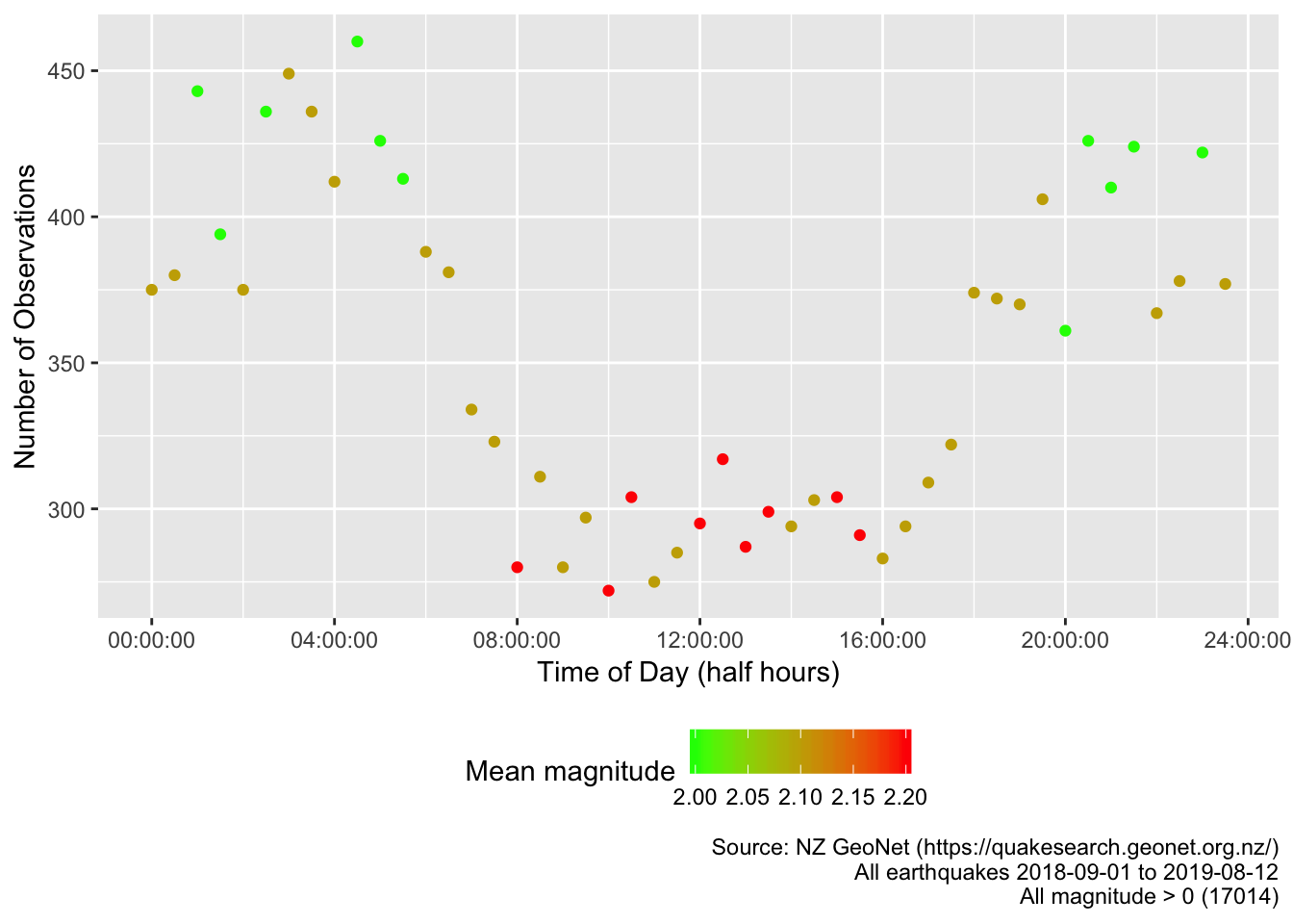
To answer this we plot all earthquakes where magnitude > 0.
plotDT <- dt[magnitude > 0, .(nObs = .N,
                 meanMag = mean(magnitude)), keyby = .(halfHour)]

myCaption <- paste0("Source: NZ GeoNet (https://quakesearch.geonet.org.nz/)\nAll earthquakes ",
                    min(lubridate::date(dt$origintime)), " to ", max(lubridate::date(dt$origintime))
                    )

p <- ggplot2::ggplot(plotDT, aes(x = halfHour,
                                 y = nObs,
                                 colour = round(meanMag,1)
                                 )
                     ) +
  geom_point() +
  labs(x = "Time of Day (half hours)",
       y = "Number of Observations",
       caption = paste0(myCaption,
                        "\nAll magnitude > 0 (", nrow(dt[magnitude > 0]), ")")) +
  scale_color_continuous(low = "green", high = "red", name = "Mean magnitude") +
  theme(legend.position="bottom")

p
Figure 3.1: Number of earthquakes by time of day
Figure 3.1 suggests more occur (or at least are detected) at night. Really? But there is a little clue in the colour of the points - the mean magnitude is higher during the day. This seems unlikely.
4 Q2: Are stronger earthquakes more likely to occur during the day?
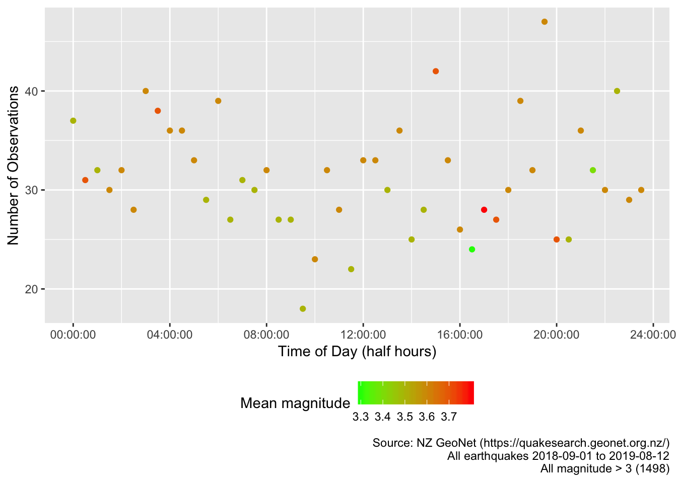
To answer this we plot all earthquakes where magnitude > 3.
plotDT <- dt[magnitude > 3, .(nObs = .N,
                 meanMag = mean(magnitude)), keyby = .(halfHour)]

p <- ggplot2::ggplot(plotDT, aes(x = halfHour,
                                 y = nObs,
                                 colour = round(meanMag,1)
                                 )
                     ) +
  geom_point() +
  labs(x = "Time of Day (half hours)",
       y = "Number of Observations",
       caption = paste0(myCaption,
                        "\nAll magnitude > 3 (", nrow(dt[magnitude > 3]), ")")
                        ) +
  scale_color_continuous(low = "green", high = "red", name = "Mean magnitude") +
  theme(legend.position="bottom")

p
Figure 4.1: Number of earthquakes by time of day (magnitude > 3)
This suggests that it is just easier to detect lower magnitude earthquakes at night when people are asleep, there are no trucks on the roads etc.
5 Q3: Are stronger earthquakes more likely during the day?
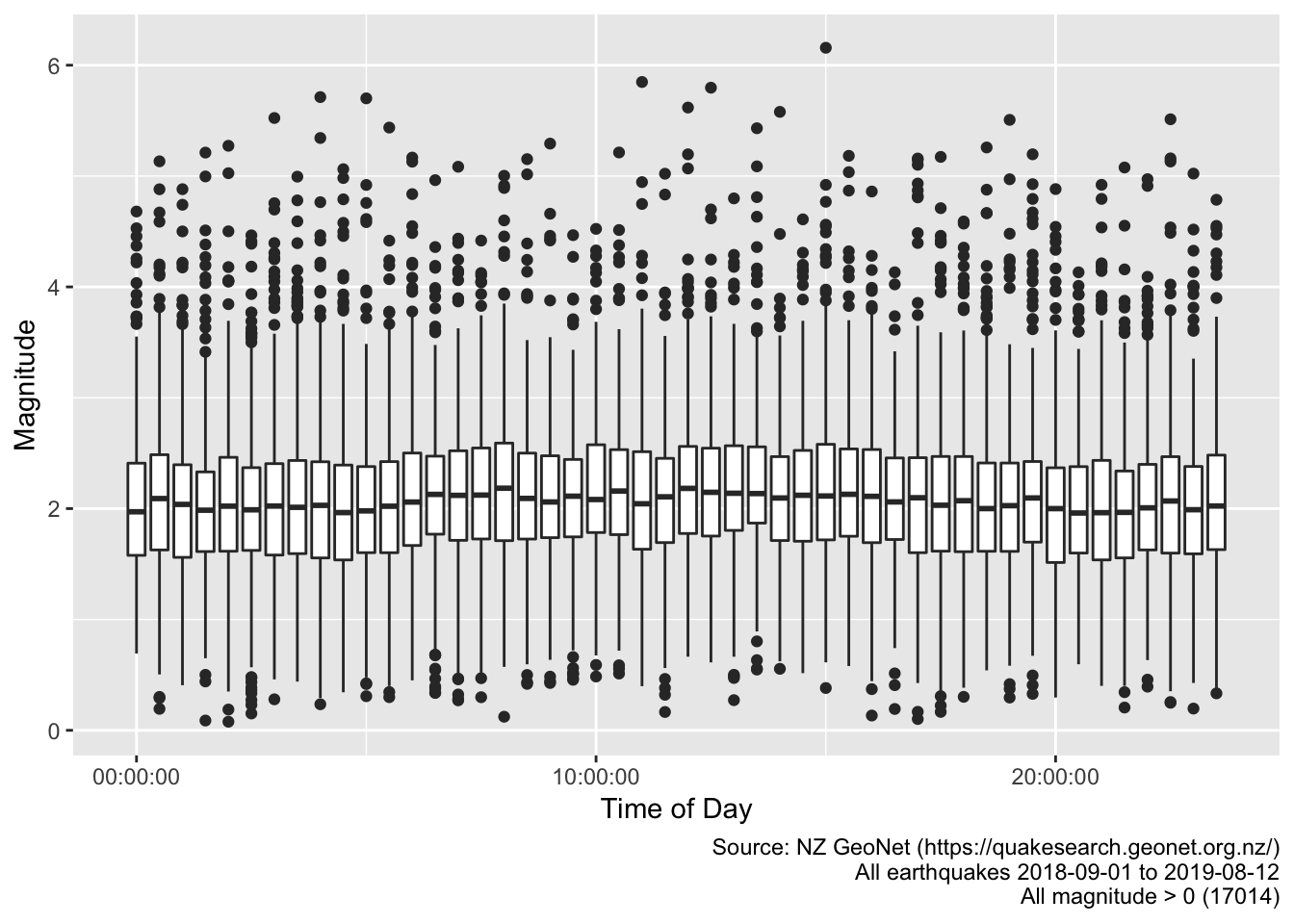
Just to check:
p <- ggplot2::ggplot(dt[magnitude > 0], aes(x = halfHour, y = magnitude, group = halfHour)) +
  geom_boxplot() +
  labs(x = "Time of Day",
       y = "Magnitude",
       caption = paste0(myCaption,
                        "\nAll magnitude > 0 (", nrow(dt[magnitude > 0]), ")")
                        ) +
  theme(legend.position="bottom")
p
Figure 5.1: Box plot of magnitude of earthquakes by time of day
No they are not.
6 Data Annex
Original data as loaded from https://quakesearch.geonet.org.nz/csv?bbox=163.95996,-49.18170,182.63672,-32.28713&startdate=2018-09-01&enddate=2019-08-13:
skimr::skim(origDT) # original data## Skim summary statistics
## n obs: 20498
## n variables: 21
##
## ── Variable type:character ───────────────────────────────────────────────────────────────────────────────────────
## variable missing complete n min max empty n_unique
## depthtype 16390 4108 20498 13 17 0 2
## earthmodel 33 20465 20498 3 8 0 4
## evaluationmethod 33 20465 20498 6 9 0 2
## evaluationmode 0 20498 20498 6 9 0 2
## evaluationstatus 3229 17269 20498 9 11 0 2
## eventtype 3161 17337 20498 9 27 0 6
## magnitudetype 0 20498 20498 1 6 0 5
## publicid 0 20498 20498 11 11 0 20498
##
## ── Variable type:numeric ─────────────────────────────────────────────────────────────────────────────────────────
## variable missing complete n mean sd p0
## azimuthalgap 0 20498 20498 139.05 66.85 0
## depth 0 20498 20498 42.09 56.41 0
## latitude 0 20498 20498 -39.7 2.16 -48.91
## longitude 0 20498 20498 170.28 42.41 -180
## magnitude 0 20498 20498 2.08 0.71 -0.15
## magnitudestationcount 0 20498 20498 9.6 8.83 1
## magnitudeuncertainty 0 20498 20498 0.0034 0.033 0
## minimumdistance 0 20498 20498 0.33 0.6 0
## originerror 0 20498 20498 0.53 0.34 0.0051
## usedphasecount 0 20498 20498 22.86 10.88 0
## usedstationcount 0 20498 20498 16.73 9.04 0
## p25 p50 p75 p100 hist
## 87.22 123.61 180.26 353.55 ▁▇▇▅▃▂▁▁
## 7.32 19.94 42.51 671.26 ▇▁▁▁▁▁▁▁
## -40.87 -39.34 -38.39 -32.29 ▁▁▁▃▇▅▁▁
## 174.44 175.85 176.9 180 ▁▁▁▁▁▁▁▇
## 1.66 2.04 2.42 6.7 ▁▃▇▃▁▁▁▁
## 6 7 11 151 ▇▁▁▁▁▁▁▁
## 0 0 0 1.06 ▇▁▁▁▁▁▁▁
## 0.085 0.15 0.31 5.95 ▇▁▁▁▁▁▁▁
## 0.33 0.45 0.61 10.42 ▇▁▁▁▁▁▁▁
## 16 20 26 132 ▃▇▁▁▁▁▁▁
## 11 14 19 119 ▇▆▁▁▁▁▁▁
##
## ── Variable type:POSIXct ─────────────────────────────────────────────────────────────────────────────────────────
## variable missing complete n min max median
## modificationtime 0 20498 20498 2018-09-01 2019-08-14 2019-03-16
## origintime 0 20498 20498 2018-09-01 2019-08-12 2019-03-15
## n_unique
## 20497
## 204967 R packages used
- base R (R Core Team 2016)
- data.table (Dowle et al. 2015) - for data munching
- drake (Landau 2019) - for data pre-loading and caching
- ggplot2 (Wickham 2009) - for plots
- hms (Müller 2018) - for time munching
- kableExtra (Zhu 2018) - for nice tables
- lubridate (Grolemund and Wickham 2011) - for dateTime munching
- readr (Wickham, Hester, and Francois 2016) - for data download & parsing
- skimr (Arino de la Rubia et al. 2017) - for data description
References
Arino de la Rubia, Eduardo, Hao Zhu, Shannon Ellis, Elin Waring, and Michael Quinn. 2017. Skimr: Skimr. https://github.com/ropenscilabs/skimr.
Dowle, M, A Srinivasan, T Short, S Lianoglou with contributions from R Saporta, and E Antonyan. 2015. Data.table: Extension of Data.frame. https://CRAN.R-project.org/package=data.table.
Grolemund, Garrett, and Hadley Wickham. 2011. “Dates and Times Made Easy with lubridate.” Journal of Statistical Software 40 (3): 1–25. http://www.jstatsoft.org/v40/i03/.
Landau, William Michael. 2019. Drake: A Pipeline Toolkit for Reproducible Computation at Scale. https://CRAN.R-project.org/package=drake.
Müller, Kirill. 2018. Hms: Pretty Time of Day. https://CRAN.R-project.org/package=hms.
R Core Team. 2016. R: A Language and Environment for Statistical Computing. Vienna, Austria: R Foundation for Statistical Computing. https://www.R-project.org/.
Wickham, Hadley. 2009. Ggplot2: Elegant Graphics for Data Analysis. Springer-Verlag New York. http://ggplot2.org.
Wickham, Hadley, Jim Hester, and Romain Francois. 2016. Readr: Read Tabular Data. https://CRAN.R-project.org/package=readr.
Zhu, Hao. 2018. KableExtra: Construct Complex Table with ’Kable’ and Pipe Syntax. https://CRAN.R-project.org/package=kableExtra.